
Very recently, Thomas Piketty’s new book, Capital in the Twenty–First Century, has been widely commented and has elicited a lot of reactions. Particularly in the United States. The theory (of inequality due to capital accumulation) advanced by the author is that the returns on invested capital (r) rises faster than economic growth (g) and written in the (already famous) formulation r>g, in the context of rising proportion of capital incomes in the total income and of capital incomes being more unequally distributed than labor incomes. This mechanism creates an ever-increasing trend of income inequality, particularly found among the top 1%, although the evidence for diminishing return of capital accumulation, powerful enough that further capital accumulation will cause a decline in net capital income rather than an expansion, considerably weakens this claim (Rognlie, 2014). But the theoretical problems with Piketty’s fundamental laws of capitalism will be covered in details in a later post.
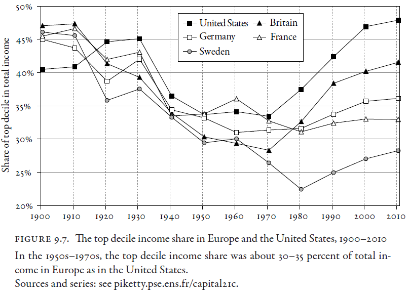
The following graphs, showing the share of top decile, top 1 percent, and top 1 thousandth in total income, for the US, and some European countries, illustrate the inequality problem pointed out by Piketty :
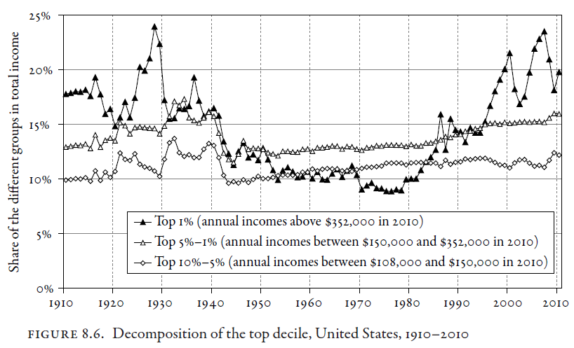
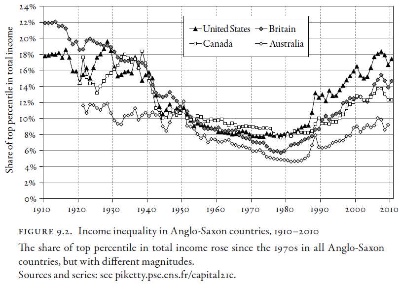
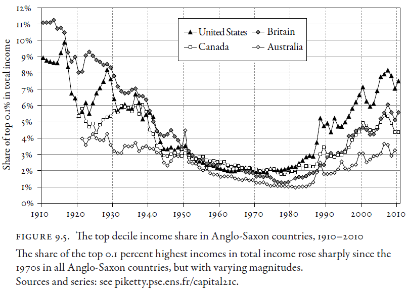
An interesting pattern is clearly visible. Too much, perhaps. We look at the large increase in the top 1% (or 0.1%) during the 1920s, and the large drop right after the 1929 crisis (Rothbard, 1963). There is another large rise in the top 1% during the 1980s (coinciding with Reagan’s administration) but stopped during the early 1990s, when a recession hit the U.S. (Hughes, 1997). We also see that the same top 1% peaks at 2000 and 2007, and then drop violently just after those respective years. It seems clear that the pattern of rise/decline in the top 1% is related with the period of economic boom, each generating their bubbles, and allow for substantial capital gains on stocks. The kind of events austrian economists always argued was caused by monetary (over)expansion, either they side with the 100% reserve banking or the free banking.
Curiously, the top decile seems to have increased since 1970s in both the UK and US. Given the other graphs shown by Piketty, there is no such tendency, especially for the US. The increase in inequality (or the top incomes) was slight and probably negligible in the 1970s but became quite substantial since the early 1980s, under the Reagan administration (and Thatcher for the UK). They cannot be responsible for the trend going from 1980s to 2010 however, as their administration lasted for only 8 years or so. It seems that the top income tax rates that has greatly diminished between 1980 and 1990, (70-75% down to 30-40%) remained as low as around 40% for both UK and US between 1990 and 2010. See Piketty & Saez (2013, Figure 5). Lane Kenworthy argues however that tax cut is an unlikely candidate for the increase in inequality.

Besides, something may have actually happened in the early 1970s. David Howden shows that the ratio of average to minimum wage increased since this period. Kopczuk et al. (2010) report that the earnings Gini coefficient increased since the early 1970s in the US. Also, a study by one of the EMP teams led by Isaacs et al. (2008) shows that from 1947 to 1973, the rate of growth of the typical family’s income was unusually rapid, roughly doubling in a generation’s time. However, since 1973 the increase over a generation’s time has been much smaller, at about 20%. Furthermore, Greenstone & Looney (2007) of the Milken Institute Review, show that the median wage has stagnated or decreased whereas the average wage of US men continues to increase. This indicates that the later wages become more skew. This may well illustrate that wages improve mainly among the extremities (e.g., top incomes). These authors, nonetheless, believe it is due to the incapacity of the US people to improve educational levels to match the increasingly more demanding jobs. Finally, Scott Winship argues that although top incomes rise at the early 1980s, the slowdown in median income growth (that has contributed to the increase in inequality) begins at the early 1970s.
One obvious coincidence with this event in the early 1970s is the abandonment of the Bretton Woods accords. The dollar was not supposed to be redeemable in gold for common people but only for foreign governments, with the dollar and gold exchange being fixed at $35 the ounce. But as the U.S. keep inflating their money supply, the dollar became overvalued (and gold, thus, became undervalued). This gives rise to the phenomenon called Gresham’s law, where the bad money drives out the good money. What happened is that the United States have pyramided the dollars on top of gold while the other governments held dollars as their basic reserve and pyramided their currency on top of the dollars.
Under Bretton Woods, the United States believe that european countries would not convert the dollar into gold, with the dollars piling up abroad staying in foreign hands and to be used as reserves for inflationary pyramiding of currencies by foreign central banks. Such a system is obviously contradictory. And in order to keep the exchange rate dollar/gold at $35 an ounce, the U.S. have no other choice than to leave the gold flee the country, as the european countries decide to redeem the dollars in gold (Rothbard, 1983, pp. 250-251, 1995, pp. 295-308).
With Bretton Woods dead, governments can inflate money supply as they please. Governments like the inflation because they are the first to benefit from it. But to the extent they inflate money supply, they need to coordinate with each other in order to avoid depreciation of their own money (currency). Otherwise, the price of the local money will be devaluated in terms of other currencies, and people will change this money into stronger currencies. Because they continue to intervene, this is not a floating exchange system anymore. Governments are usually afraid of trade deficit because it implies they export less than they import due to their local money being stronger. But this is illogical, and Rothbard (1995, p. 178) explains that trade deficit is of no problem if there is no payment deficit. A strong(er) currency can attract foreigners to invest in this money, and this results in capital inflow into the country. Unfortunately, the political elites consider that being in trade deficit is considered as being a debtor while being in trade surplus is considered as being a creditor. When inflation is higher in a given country, people find harder to buy products and goods while export companies find easier to export their products because the local money has lost value relative to other monies. A foreign money can buy more of their local money. Even though inflation is kept at “reasonable” rates by central banks, inflation will surely be of lower levels under the gold standard. Here’s how Rothbard (1981) narrates the story :
As dollars piled up abroad and gold continued to flow outward, the United States found it increasingly difficult to maintain the price of gold at $35 an ounce in the free gold markets at London and Zurich. Thirty-five dollars an ounce was the keystone of the system, and while American citizens have been barred since 1934 from owning gold anywhere in the world, other citizens have enjoyed the freedom to own gold bullion and coin. Hence, one way for individual Europeans to redeem their dollars in gold was to sell their dollars for gold at $35 an ounce in the free gold market. As the dollar kept inflating and depreciating, and as American balance of payments deficits continued, Europeans and other private citizens began to accelerate their sales of dollars into gold. In order to keep the dollar at $35 an ounce, the United States government was forced to leak out gold from its dwindling stock to support the $35 price at London and Zurich. …
All pro-paper economists, from Keynesians to Friedmanites, were now confident that gold would disappear from the international monetary system; cut off from its “support” by the dollar, these economists all confidently predicted, the free-market gold price would soon fall below $35 an ounce, and even down to the estimated “industrial” nonmonetary gold price of $10 an ounce. Instead, the free price of gold, never below $35, had been steadily above $35, and by early 1973 had climbed to around $125 an ounce, a figure that no pro-paper economist would have thought possible as recently as a year earlier. …
The swollen supply of Eurodollars, combined with the continued inflation and the removal of gold backing, drove the free-market gold price up to $215 an ounce. And as the overvaluation of the dollar and the undervaluation of European and Japanese hard money became increasingly evident, the dollar finally broke apart on the world markets in the panic months of February–March 1973. It became impossible for West Germany, Switzerland, France and the other hard money countries to continue to buy dollars in order to support the dollar at an overvalued rate. In little over a year, the Smithsonian system of fixed exchange rates without gold had smashed apart on the rocks of economic reality. …
But it became clear all too soon that all is far from well in the current international monetary system. The long-run problem is that the hard-money countries will not sit by forever and watch their currencies become more expensive and their exports hurt for the benefit of their American competitors. If American inflation and dollar depreciation continues, they will soon shift to the competing devaluation, exchange controls, currency blocs, and economic warfare of the 1930s. But more immediate is the other side of the coin: the fact that depreciating dollars means that American imports are far more expensive, American tourists suffer abroad, and cheap exports are snapped up by foreign countries so rapidly as to raise prices of exports at home (e.g., the American wheat-and-meat price inflation). So that American exporters might indeed benefit, but only at the expense of the inflation-ridden American consumer. The crippling uncertainty of rapid exchange rate fluctuations was brought starkly home to Americans with the rapid plunge of the dollar in foreign exchange markets in July 1973.
Why is monetary (over)expansion relevant here ? We need to think about the Cantillon effect, which states that the first persons having received and spent the newly created money will be those who benefit from money creation, because they have spent money before price increases, under the inflated demand for goods. The other people will receive the money after it has been spent and, thus, after the increase in prices. Certainly, those being the closest to the source of credit are more likely to be richer, those people who can afford loans to make investments. On the other hand, poor(er) people receive the new money in the form of pay and salary, i.e., after the increase in prices. Furthermore, poor people save less money. But also, they don’t hedge their savings against financial disasters. Richer people, however, save and hedge. This is an important detail. Since the era of fluctuating fiat money, the economies are much more subjected to financial instability. Certainly, financial planning is more likely to be practiced by wealthy, high-IQ, and rich people.
Under these conditions, people who merely live of their wage, and not of wage+capital, will be increasingly ruined. This is relevant to Piketty’s theory because it is based on the assumption that the role of capital becomes increasingly important behind income inequality. There is something else than 1973 or the inflation. And Leopold (2012) shows what it is :

It is obvious that the financial/nonfinancial gap happens well after Bretton Woods. At the same time, during the 1970s, multiple crises hit the U.S. It is hardly conceivable that financial markets will bloom during periods of recession. On the other hand, deregulation with respect to financial market unfolds since this very period of early 1980s.
And this is the hypothesis favored by Wuergler (2009) to explain this phenomenon. Deregulation favors asset bubbles, which increases the opportunity set of skilled individuals in financial intermediation, causing income inequality. But, in fact, it should be best understood in terms of interaction between deregulation and monetary over-expansion. That is, the rise in inequality owing to financial markets is due to the simultaneous presence of both factors. Obviously, eliminating monetary over-expansion will also annihilate much of this trend. At the same time, this means when we are in presence of deregulation and monetary expansion we are expected to see the countries having more deregulated financial markets will also experience more financial/nonfinancial wage gaps growth. This is exactly what Wuergler (2009) finds out. The trend is depicted below :


Similar findings come from Philippon & Reshef (2009). We notice some sort of increasing trends in both finance/non-finance wage gaps and financial intermediation since the 1980s for UK and US, but not really for Germany and France. The author argues this is due to the massive deregulation operated in these countries, under Ronald Reagan and Margaret Thatcher. Given this picture, one should not be surprised to find out that the GDP share of the US financial industry has increased dramatically since the 1980s (Philippon, 2008, Figure 1) although it also tends to be driven by the boom-bust cycle.
What happened perfectly illustrates the austrian malinvestment process, which results in crowding-out effects. And Wuergler recognizes that the growth of financial market requires more and more complex jobs. For example, with respect to CDO/CDS in the recent US subprime crisis, financial institutions had to employ hoards of mathematicians, IT engineers and quantitative finance specialists to handle these highly complex transactions.
One of the prediction of ABCT (although non-exclusive to it) is that these trends in wages must be matched by similar trends in education and job complexity related to the financial industry. But this brings us to the all other things equal assumption. And yet, Philippon & Reshef (2009) confirmed the prediction. As depicted in Figures 1 & 3, the complexity and education related to financial industry both closely match the trends in financial wages for the period of 1910-2010.


But the authors argue this relationship is the result of deregulation. When they use time series regression for relative education and relative wages (in dependent variables) with deregulation index, ratio of financial patents over total patents, IPO share of market capitalization, default rate (all american corporates), time trend, in independent variables (all having a lag of t-5 years), it appeared that deregulation had the strongest effect on either relative education or relative wages. In regression equations having only time trend and deregulation for independent variables, the model has an R² of 0.89 and 0.83 for education and wages (to get the unbiased effect size, R² should better be square rooted). The effect of deregulation is robust to the addition of other independent variables. Since regression partials out independent variables’ total effect, their effect can be hidden into the common effect not evaluated by regression coefficients, but unless they have causal effect on deregulation, and not the reverse, it seems unlikely that their effects are under-estimated relative to deregulation. They perform another regression using a Deregulation Index (t-5) varying by (financial) sectors, and they hold sectors and year effects constant. They add another predictor variables, Share of IT in Capital Stock of Subsector (t-5). The effect of deregulation was 1.5 times stronger than IT.
In support for the hypothesis of causal role concerning (de)regulation, they affirm (pp. 21-22) that financial wage began to change not just at the time the crises hit the economy (e.g., 1929-33 and 1970-80s) but after new regulations were enforced (e.g., 1934). Furthermore, in the 1929 crisis, regulations were tightened and financial wages went down, whereas during the 1973-1981, regulations were loosened, and financial wages went up. They also believe the role of IT and software to be limited because the IT share in the capital stock of Insurance and in Credit Intermediation has increased just as much as Other Finance, while the wage gains are much more modest.
One could argue the evidence displayed so far is not the most compelling because inequality, according to Piketty, is mainly due to the top 1 percent and more. Upon close examination of the Statistics of Income (SOI) division of the Internal Revenue Service, Bakija et al. (2012) highlight the importance of financial and real estate jobs in the increase of inequality owing to incomes gains going to the 1 and 0.1 top percent. They coincide with the periods of boom. Still, other jobs have seen large gains as well.


This is not to say that financial market must necessarily cause income inequality. But given the episodes of repeated monetary (over)expansions, they should. Financial market, under this situation, may not be positively associated with growth anymore. For instance, Capelle-Blancard & Labonne (2011) use regressions to model the effect of financial deepening (i.e., activities) on economic growth. The size of the financial sectors is based on inputs rather than outputs, specifically, the number of employees divided by total workforce, and ratio of private credit divided by the number of employees in financial sectors. They also use traditional measures of financial activity, such as the ratio of private credit to GDP, and ratio of liquid liabilities to GDP, and ratio of commercial bank credits to total credits (commercial + central banks). The period covers 1970-2008 for 24 OECD countries. Their first-step regression model involves financial deepening, GDP per capita and initial level of human capital, and the second-step model adds inflation, government size (expenses) and the ratio of the sum of importations and exportations to GDP. They also include a variable financial_sector*crisis. There is no strong evidence for an effect of financial activities on growth. The authors suggest the cause to be the excessive credit growth and misallocations of talents (as explicited by Philippon & Reshef, 2009).
Bonnet et al. (2014) show that the increase in the share of capital in total income is entirely accounted for by housing capital (more exactly, a rise in housing prices). When housing capital is measured in rent instead of housing prices, there is no increasing trend for capital/income ratio. The reason to rely of rent is because rent is more inclusive and accurate. For example, landlords earn incomes from renting, whereas owner-occupiers do not receive any income but still receive an implicit return as rent that is saved or economized by these owner-occupiers.
Overall, there is some indication that financial and housing boom is mainly responsible for the increasing inequality documented by Piketty and others. If the boom is the result of monetary (over)expansion hypothesized by the ABCT, it is not a problem inherent to free market or capitalism. It is possible indeed to mitigate income inequality by reinforcing financial regulation but it is also possible to attack the root causes by reestablishing sound money.
References :
Atkinson, A. B., Piketty, T., & Saez, E. (2011). Top Incomes in the Long Run of History. Journal of Economic Literature, 49(1), 3-71.
Bakija, J., Cole, A., & Heim, B. T. (2012). Jobs and income growth of top earners and the causes of changing income inequality: Evidence from US tax return data. Williamstown: Williams College.
Bonnet, O., Bono, P. H., Chapelle, G., & Wasmer, E. (2014). Does housing capital contribute to inequality? A comment on Thomas Piketty’s Capital in the 21st Century (No. 2014-07). Sciences Po Departement of Economics.
Capelle-Blancard, G., & Labonne, C. (2011). More bankers, more growth? Evidence from OECD countries. Evidence from OECD Countries (December 21, 2011).
Greenstone, Michael, & Looney, Adam (2007). Trends: Reduced Earnings for Men in America. Hamilton Project.
Isaacs, J. B., Sawhill, I. V., & Haskins, R. (2008). Getting Ahead or Losing Ground: Economic Mobility in America. Brookings Institution.
Leopold, L. (2012). How to Make a Million Dollars an Hour: Why Hedge Funds Get Away with Siphoning Off America’s Wealth. John Wiley & Sons.
Philippon, T. (2008). The Evolution of the US Financial Industry from 1860 to 2007: Theory and evidence. mimeograph, New York University.
Philippon, T., & Reshef, A. (2009). Wages and Human Capital in the U.S. Financial Industry: 1909-2006 (No. w14644). National Bureau of Economic Research.
Piketty, T. (2014). Capital in the 21st Century. Harvard University Press.
Piketty, T., & Saez, E. (2013). Top Incomes and the Great Recession: Recent Evolutions and Policy Implications. IMF Economic review, 61(3), 456-478.
Rognlie Matthew (2014). A note on Piketty and diminishing returns to capital.
Rothbard, M. N. (1981). What Has Government Done to Our Money?. Ludwig von Mises Institute.
Rothbard, M. N. (1983). Mystery of Banking. The. Ludwig von Mises Institute.
Rothbard, M. N. (1995). Making economic sense. Ludwig von Mises Institute.
Wuergler, T. (2009). Of bubbles and bankers: The impact of financial booms on labor markets. Institute for Empirical Research in Economics, University of Zurich.
